Intraday Factor
In this notebook we use Alphalens to analyse the performance of an intraday factor, which is computed daily but the stocks are bought at marker open and sold at market close with no overnight positions.
Imports & Settings
[2]:
import warnings
warnings.filterwarnings('ignore')
[3]:
import alphalens
import pandas as pd
[4]:
%matplotlib inline
Loading Data
Below is a simple mapping of tickers to sectors for a small universe of large cap stocks.
[5]:
sector_names = {
    0 : "information_technology",
    1 : "financials",
    2 : "health_care",
    3 : "industrials",
    4 : "utilities",
    5 : "real_estate",
    6 : "materials",
    7 : "telecommunication_services",
    8 : "consumer_staples",
    9 : "consumer_discretionary",
    10 : "energy"
}

ticker_sector = {
    "ACN" : 0, "ATVI" : 0, "ADBE" : 0, "AMD" : 0, "AKAM" : 0, "ADS" : 0, "GOOGL" : 0, "GOOG" : 0,
    "APH" : 0, "ADI" : 0, "ANSS" : 0, "AAPL" : 0, "AMAT" : 0, "ADSK" : 0, "ADP" : 0, "AVGO" : 0,
    "AMG" : 1, "AFL" : 1, "ALL" : 1, "AXP" : 1, "AIG" : 1, "AMP" : 1, "AON" : 1, "AJG" : 1, "AIZ" : 1, "BAC" : 1,
    "BK" : 1, "BBT" : 1, "BRK.B" : 1, "BLK" : 1, "HRB" : 1, "BHF" : 1, "COF" : 1, "CBOE" : 1, "SCHW" : 1, "CB" : 1,
    "ABT" : 2, "ABBV" : 2, "AET" : 2, "A" : 2, "ALXN" : 2, "ALGN" : 2, "AGN" : 2, "ABC" : 2, "AMGN" : 2, "ANTM" : 2,
    "BCR" : 2, "BAX" : 2, "BDX" : 2, "BIIB" : 2, "BSX" : 2, "BMY" : 2, "CAH" : 2, "CELG" : 2, "CNC" : 2, "CERN" : 2,
    "MMM" : 3, "AYI" : 3, "ALK" : 3, "ALLE" : 3, "AAL" : 3, "AME" : 3, "AOS" : 3, "ARNC" : 3, "BA" : 3, "CHRW" : 3,
    "CAT" : 3, "CTAS" : 3, "CSX" : 3, "CMI" : 3, "DE" : 3, "DAL" : 3, "DOV" : 3, "ETN" : 3, "EMR" : 3, "EFX" : 3,
    "AES" : 4, "LNT" : 4, "AEE" : 4, "AEP" : 4, "AWK" : 4, "CNP" : 4, "CMS" : 4, "ED" : 4, "D" : 4, "DTE" : 4,
    "DUK" : 4, "EIX" : 4, "ETR" : 4, "ES" : 4, "EXC" : 4, "FE" : 4, "NEE" : 4, "NI" : 4, "NRG" : 4, "PCG" : 4,
    "ARE" : 5, "AMT" : 5, "AIV" : 5, "AVB" : 5, "BXP" : 5, "CBG" : 5, "CCI" : 5, "DLR" : 5, "DRE" : 5,
    "EQIX" : 5, "EQR" : 5, "ESS" : 5, "EXR" : 5, "FRT" : 5, "GGP" : 5, "HCP" : 5, "HST" : 5, "IRM" : 5, "KIM" : 5,
    "APD" : 6, "ALB" : 6, "AVY" : 6, "BLL" : 6, "CF" : 6, "DWDP" : 6, "EMN" : 6, "ECL" : 6, "FMC" : 6, "FCX" : 6,
    "IP" : 6, "IFF" : 6, "LYB" : 6, "MLM" : 6, "MON" : 6, "MOS" : 6, "NEM" : 6, "NUE" : 6, "PKG" : 6, "PPG" : 6,
    "T" : 7, "CTL" : 7, "VZ" : 7,
    "MO" : 8, "ADM" : 8, "BF.B" : 8, "CPB" : 8, "CHD" : 8, "CLX" : 8, "KO" : 8, "CL" : 8, "CAG" : 8,
    "STZ" : 8, "COST" : 8, "COTY" : 8, "CVS" : 8, "DPS" : 8, "EL" : 8, "GIS" : 8, "HSY" : 8, "HRL" : 8,
    "AAP" : 9, "AMZN" : 9, "APTV" : 9, "AZO" : 9, "BBY" : 9, "BWA" : 9, "KMX" : 9, "CCL" : 9,
    "APC" : 10, "ANDV" : 10, "APA" : 10, "BHGE" : 10, "COG" : 10, "CHK" : 10, "CVX" : 10, "XEC" : 10, "CXO" : 10,
    "COP" : 10, "DVN" : 10, "EOG" : 10, "EQT" : 10, "XOM" : 10, "HAL" : 10, "HP" : 10, "HES" : 10, "KMI" : 10
}
YFinance Download
[6]:
import yfinance as yf
import pandas_datareader.data as web
yf.pdr_override()

tickers = list(ticker_sector.keys())
df = web.get_data_yahoo(tickers, start='2017-01-01',  end='2017-06-01')
df.index = pd.to_datetime(df.index, utc=True)
[*********************100%***********************]  182 of 182 completed

19 Failed downloads:
- CHK: Data doesn't exist for startDate = 1483250400, endDate = 1496293200
- BF.B: No data found for this date range, symbol may be delisted
- BRK.B: No data found, symbol may be delisted
- MON: Data doesn't exist for startDate = 1483250400, endDate = 1496293200
- CELG: No data found, symbol may be delisted
- APC: No data found, symbol may be delisted
- ARNC: Data doesn't exist for startDate = 1483250400, endDate = 1496293200
- CBG: No data found for this date range, symbol may be delisted
- CTL: No data found, symbol may be delisted
- BCR: No data found for this date range, symbol may be delisted
- DWDP: No data found, symbol may be delisted
- BHF: Data doesn't exist for startDate = 1483250400, endDate = 1496293200
- GGP: No data found for this date range, symbol may be delisted
- CXO: No data found, symbol may be delisted
- HCP: No data found, symbol may be delisted
- DPS: No data found for this date range, symbol may be delisted
- AGN: No data found, symbol may be delisted
- BBT: No data found, symbol may be delisted
- BHGE: No data found, symbol may be delisted
[7]:
df = df.stack()
df.index.names = ['date', 'asset']
df.info()
<class 'pandas.core.frame.DataFrame'>
MultiIndex: 16789 entries, (Timestamp('2017-01-03 00:00:00+0000', tz='UTC'), 'A') to (Timestamp('2017-05-31 00:00:00+0000', tz='UTC'), 'XOM')
Data columns (total 6 columns):
 #   Column     Non-Null Count  Dtype
---  ------     --------------  -----
 0   Adj Close  16789 non-null  float64
 1   Close      16789 non-null  float64
 2   High       16789 non-null  float64
 3   Low        16789 non-null  float64
 4   Open       16789 non-null  float64
 5   Volume     16789 non-null  float64
dtypes: float64(6)
memory usage: 842.6+ KB
Factor Computation
Our example factor ranks the stocks based on their overnight price gap (yesterday close to today open price). We’ll see if the factor has some alpha or if it is pure noise.
[8]:
available_tickers = df.index.unique('asset')
ticker_sector = {k: v for k, v in ticker_sector.items() if k in available_tickers}
[9]:
today_open = df.loc[:, 'Open'].unstack('asset')
today_close = df.loc[:, 'Close'].unstack('asset')
yesterday_close = today_close.shift(1)
[10]:
factor = (today_open - yesterday_close) / yesterday_close
The pricing data passed to alphalens should contain the entry price for the assets so it must reflect the next available price after a factor value was observed at a given timestamp. Those prices must not be used in the calculation of the factor values for that time. Always double check to ensure you are not introducing lookahead bias to your study.
The pricing data must also contain the exit price for the assets, for period 1 the price at the next timestamp will be used, for period 2 the price after 2 timestamps will be used and so on.
There are no restrinctions/assumptions on the time frequencies a factor should be computed at and neither on the specific time a factor should be traded (trading at the open vs trading at the close vs intraday trading), it is only required that factor and price DataFrames are properly aligned given the rules above.
In our example, we want to buy the stocks at marker open, so the need the open price at the exact timestamps as the factor valules, and we want to sell the stocks at market close so we will add the close prices too, which will be used to compute period 1 forward returns as they appear just after the factor values timestamps. The returns computed by Alphalens will therefore be based on the difference between open to close assets prices.
If we had other prices we could compute other period returns, for example one hour after market open and 2 hours and so on. We could have added those prices right after the open prices and instruct Alphalens to compute 1, 2, 3… periods too and not only period 1 like in this example.
Data Formatting
Time Adjustments
[11]:
# Fix time as Yahoo doesn't set it
today_open.index += pd.Timedelta('9h30m')
today_close.index += pd.Timedelta('16h')
# pricing will contain both open and close
pricing = pd.concat([today_open, today_close]).sort_index()
[12]:
pricing.head()
[12]:
| asset | A | AAL | AAP | AAPL | ABBV | ABC | ABT | ACN | ADBE | ADI | ... | NUE | PCG | PKG | PPG | SCHW | STZ | T | VZ | XEC | XOM |
|---|---|---|---|---|---|---|---|---|---|---|---|---|---|---|---|---|---|---|---|---|---|
| date | |||||||||||||||||||||
| 2017-01-03 09:30:00+00:00 | 45.930000 | 47.279999 | 170.779999 | 28.950001 | 62.919998 | 78.510002 | 38.630001 | 117.379997 | 103.430000 | 72.599998 | ... | 59.740002 | 60.810001 | 85.160004 | 95.430000 | 40.049999 | 155.009995 | 42.689999 | 53.959999 | 137.529999 | 90.940002 |
| 2017-01-03 16:00:00+00:00 | 46.490002 | 46.299999 | 170.600006 | 29.037500 | 62.410000 | 82.610001 | 39.049999 | 116.459999 | 103.480003 | 72.510002 | ... | 59.610001 | 60.369999 | 85.000000 | 95.250000 | 40.200001 | 154.750000 | 43.020000 | 54.580002 | 138.789993 | 90.889999 |
| 2017-01-04 09:30:00+00:00 | 46.930000 | 46.630001 | 170.369995 | 28.962500 | 62.639999 | 82.599998 | 39.060001 | 116.910004 | 103.739998 | 72.769997 | ... | 59.759998 | 60.610001 | 85.440002 | 95.709999 | 40.400002 | 157.149994 | 42.939999 | 54.549999 | 138.479996 | 91.120003 |
| 2017-01-04 16:00:00+00:00 | 47.099998 | 46.700001 | 172.000000 | 29.004999 | 63.290001 | 84.660004 | 39.360001 | 116.739998 | 104.139999 | 72.360001 | ... | 61.250000 | 60.590000 | 86.370003 | 97.269997 | 41.220001 | 157.990005 | 42.770000 | 54.520000 | 138.500000 | 89.889999 |
| 2017-01-05 09:30:00+00:00 | 47.049999 | 46.520000 | 170.869995 | 28.980000 | 63.380001 | 84.379997 | 39.240002 | 116.980003 | 104.129997 | 72.410004 | ... | 61.119999 | 60.660000 | 86.370003 | 96.459999 | 40.970001 | 150.550003 | 42.849998 | 54.779999 | 138.500000 | 90.190002 |
5 rows × 163 columns
Align Factor & Price
[13]:
# Align factor to open price
factor.index += pd.Timedelta('9h30m')
factor = factor.stack()
factor.index = factor.index.set_names(['date', 'asset'])
[14]:
factor.unstack().head()
[14]:
| asset | A | AAL | AAP | AAPL | ABBV | ABC | ABT | ACN | ADBE | ADI | ... | NUE | PCG | PKG | PPG | SCHW | STZ | T | VZ | XEC | XOM |
|---|---|---|---|---|---|---|---|---|---|---|---|---|---|---|---|---|---|---|---|---|---|
| date | |||||||||||||||||||||
| 2017-01-04 09:30:00+00:00 | 0.009464 | 0.007127 | -0.001348 | -0.002583 | 0.003685 | -0.000121 | 0.000256 | 0.003864 | 0.002513 | 0.003586 | ... | 0.002516 | 0.003976 | 0.005176 | 0.004829 | 0.004975 | 0.015509 | -0.001860 | -0.000550 | -0.002234 | 0.002531 |
| 2017-01-05 09:30:00+00:00 | -0.001062 | -0.003854 | -0.006570 | -0.000862 | 0.001422 | -0.003307 | -0.003049 | 0.002056 | -0.000096 | 0.000691 | ... | -0.002122 | 0.001155 | 0.000000 | -0.008327 | -0.006065 | -0.047092 | 0.001870 | 0.004769 | 0.000000 | 0.003337 |
| 2017-01-06 09:30:00+00:00 | 0.001934 | -0.000872 | -0.003258 | 0.001458 | 0.001725 | -0.001793 | 0.000000 | 0.000000 | 0.000661 | 0.003646 | ... | -0.000328 | -0.003304 | 0.000469 | 0.001569 | 0.008055 | 0.001635 | -0.015709 | -0.017753 | 0.001784 | 0.002710 |
| 2017-01-09 09:30:00+00:00 | 0.000417 | -0.004328 | 0.002535 | 0.000339 | 0.000157 | -0.002359 | 0.000245 | -0.001376 | -0.003139 | 0.000559 | ... | 0.009786 | -0.000327 | -0.003440 | -0.005649 | -0.005578 | 0.003747 | -0.000726 | -0.000751 | -0.011285 | -0.003164 |
| 2017-01-10 09:30:00+00:00 | 0.004155 | -0.001699 | -0.004896 | -0.001849 | -0.002492 | -0.004446 | 0.001718 | -0.000522 | 0.000000 | -0.000973 | ... | 0.012743 | 0.000498 | -0.000798 | -0.002906 | 0.001702 | -0.001797 | -0.003431 | 0.000190 | 0.004664 | 0.001494 |
5 rows × 163 columns
Run Alphalens
Period 1 will show returns from market open to market close while period 2 will show returns from today open to tomorrow open
Get Alphalens Input
[15]:
non_predictive_factor_data = alphalens.utils.get_clean_factor_and_forward_returns(factor,
                                                                                  pricing,
                                                                                  periods=(1,2),
                                                                                  groupby=ticker_sector,
                                                                                  groupby_labels=sector_names)
Dropped 2.9% entries from factor data: 1.0% in forward returns computation and 2.0% in binning phase (set max_loss=0 to see potentially suppressed Exceptions).
max_loss is 35.0%, not exceeded: OK!
Returns Tear Sheet
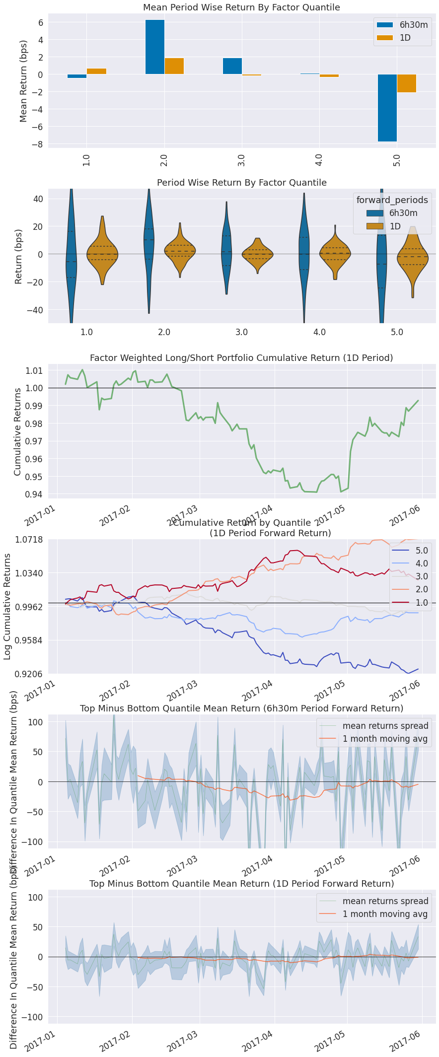
[16]:
alphalens.tears.create_returns_tear_sheet(non_predictive_factor_data)
Returns Analysis
| 6h30m | 1D | |
|---|---|---|
| Ann. alpha | 0.324 | -0.046 |
| beta | 0.177 | 0.179 |
| Mean Period Wise Return Top Quantile (bps) | -7.776 | -2.096 |
| Mean Period Wise Return Bottom Quantile (bps) | -0.445 | 0.697 |
| Mean Period Wise Spread (bps) | -7.331 | -2.795 |
<Figure size 432x288 with 0 Axes>
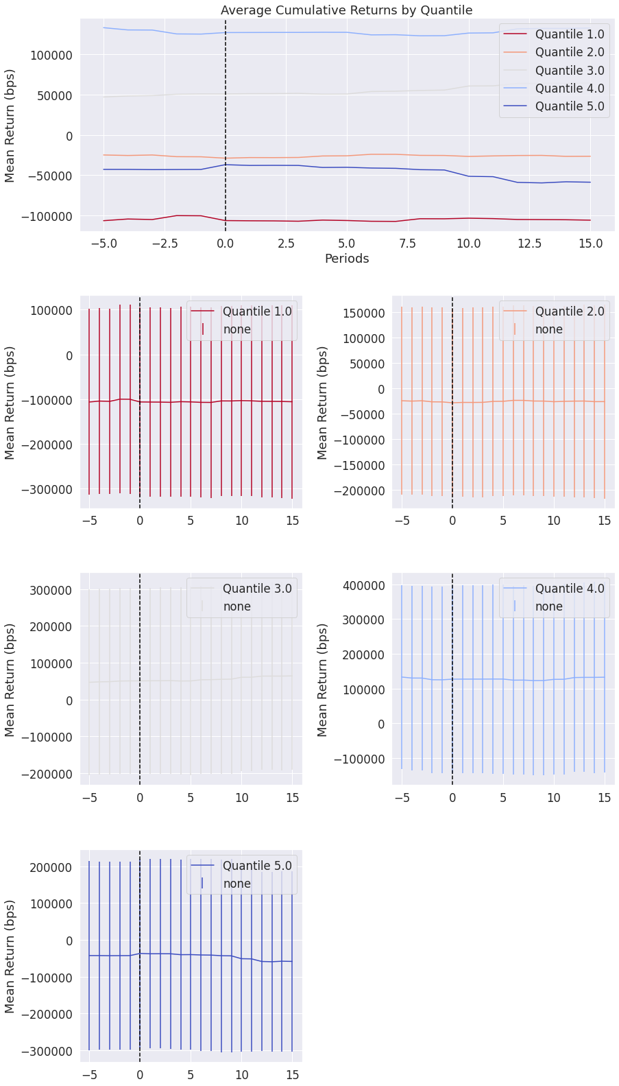
[17]:
alphalens.tears.create_event_returns_tear_sheet(non_predictive_factor_data, pricing);
<Figure size 432x288 with 0 Axes>