Pyfolio Integration — Alphalens 0.4.1post1+8.g3348e92 documentation

Imports & Settings¶

[1]:

import warnings
warnings.filterwarnings('ignore')

[2]:

import alphalens
import pyfolio
import pandas as pd

[3]:

%matplotlib inline

Load Data¶

First load some stocks data

[4]:

tickers = [ 'ACN', 'ATVI', 'ADBE', 'AMD', 'AKAM', 'ADS', 'GOOGL', 'GOOG', 'APH', 'ADI', 'ANSS', 'AAPL',
'AVGO', 'CA', 'CDNS', 'CSCO', 'CTXS', 'CTSH', 'GLW', 'CSRA', 'DXC', 'EBAY', 'EA', 'FFIV', 'FB',
'FLIR', 'IT', 'GPN', 'HRS', 'HPE', 'HPQ', 'INTC', 'IBM', 'INTU', 'JNPR', 'KLAC', 'LRCX', 'MA', 'MCHP',
'MSFT', 'MSI', 'NTAP', 'NFLX', 'NVDA', 'ORCL', 'PAYX', 'PYPL', 'QRVO', 'QCOM', 'RHT', 'CRM', 'STX',
'AMG', 'AFL', 'ALL', 'AXP', 'AIG', 'AMP', 'AON', 'AJG', 'AIZ', 'BAC', 'BK', 'BBT', 'BRK.B', 'BLK', 'HRB',
'BHF', 'COF', 'CBOE', 'SCHW', 'CB', 'CINF', 'C', 'CFG', 'CME', 'CMA', 'DFS', 'ETFC', 'RE', 'FITB', 'BEN',
'GS', 'HIG', 'HBAN', 'ICE', 'IVZ', 'JPM', 'KEY', 'LUK', 'LNC', 'L', 'MTB', 'MMC', 'MET', 'MCO', 'MS',
'NDAQ', 'NAVI', 'NTRS', 'PBCT', 'PNC', 'PFG', 'PGR', 'PRU', 'RJF', 'RF', 'SPGI', 'STT', 'STI', 'SYF', 'TROW',
'ABT', 'ABBV', 'AET', 'A', 'ALXN', 'ALGN', 'AGN', 'ABC', 'AMGN', 'ANTM', 'BCR', 'BAX', 'BDX', 'BIIB', 'BSX',
'BMY', 'CAH', 'CELG', 'CNC', 'CERN', 'CI', 'COO', 'DHR', 'DVA', 'XRAY', 'EW', 'EVHC', 'ESRX', 'GILD', 'HCA',
'HSIC', 'HOLX', 'HUM', 'IDXX', 'ILMN', 'INCY', 'ISRG', 'IQV', 'JNJ', 'LH', 'LLY', 'MCK', 'MDT', 'MRK', 'MTD',
'MYL', 'PDCO', 'PKI', 'PRGO', 'PFE', 'DGX', 'REGN', 'RMD', 'SYK', 'TMO', 'UNH', 'UHS', 'VAR', 'VRTX', 'WAT',
'MMM', 'AYI', 'ALK', 'ALLE', 'AAL', 'AME', 'AOS', 'ARNC', 'BA', 'CHRW', 'CAT', 'CTAS', 'CSX', 'CMI', 'DE',
'DAL', 'DOV', 'ETN', 'EMR', 'EFX', 'EXPD', 'FAST', 'FDX', 'FLS', 'FLR', 'FTV', 'FBHS', 'GD', 'GE', 'GWW',
'HON', 'INFO', 'ITW', 'IR', 'JEC', 'JBHT', 'JCI', 'KSU', 'LLL', 'LMT', 'MAS', 'NLSN', 'NSC', 'NOC', 'PCAR',
'PH', 'PNR', 'PWR', 'RTN', 'RSG', 'RHI', 'ROK', 'COL', 'ROP', 'LUV', 'SRCL', 'TXT', 'TDG', 'UNP', 'UAL',
'AES', 'LNT', 'AEE', 'AEP', 'AWK', 'CNP', 'CMS', 'ED', 'D', 'DTE', 'DUK', 'EIX', 'ETR', 'ES', 'EXC']

YFinance Download¶

[5]:

import yfinance as yf
import pandas_datareader.data as web
yf.pdr_override()

df = web.get_data_yahoo(tickers, start='2015-01-01',  end='2017-01-01')
df.index = pd.to_datetime(df.index, utc=True)

[*********************100%***********************]  247 of 247 completed

17 Failed downloads:
- RHT: No data found, symbol may be delisted
- JEC: No data found, symbol may be delisted
- RTN: No data found, symbol may be delisted
- BBT: No data found, symbol may be delisted
- BHF: Data doesn't exist for startDate = 1420092000, endDate = 1483250400
- AGN: No data found, symbol may be delisted
- BRK.B: No data found, symbol may be delisted
- ARNC: Data doesn't exist for startDate = 1420092000, endDate = 1483250400
- HRS: No data found, symbol may be delisted
- IR: Data doesn't exist for startDate = 1420092000, endDate = 1483250400
- CELG: No data found, symbol may be delisted
- BCR: No data found for this date range, symbol may be delisted
- STI: No data found, symbol may be delisted
- MYL: No data found, symbol may be delisted
- LUK: No data found for this date range, symbol may be delisted
- LLL: No data found, symbol may be delisted
- ETFC: No data found, symbol may be delisted

Data Formatting¶

[6]:

df = df.stack()
df.index.names = ['date', 'asset']
df.info()

<class 'pandas.core.frame.DataFrame'>
MultiIndex: 114987 entries, (Timestamp('2015-01-02 00:00:00+0000', tz='UTC'), 'A') to (Timestamp('2016-12-30 00:00:00+0000', tz='UTC'), 'XRAY')
Data columns (total 6 columns):
 #   Column     Non-Null Count   Dtype
---  ------     --------------   -----
 0   Adj Close  114987 non-null  float64
 1   Close      114987 non-null  float64
 2   High       114987 non-null  float64
 3   Low        114987 non-null  float64
 4   Open       114987 non-null  float64
 5   Volume     114987 non-null  float64
dtypes: float64(6)
memory usage: 5.7+ MB

Compute Factor¶

We’ll compute a simple mean reversion factor looking at recent stocks performance: stocks that performed well in the last 5 days will have high rank and vice versa.

[7]:

factor = df.loc[:,'Open'].unstack('asset')
factor = -factor.pct_change(5)
factor = factor.stack()

The pricing data passed to alphalens should contain the entry price for the assets so it must reflect the next available price after a factor value was observed at a given timestamp. Those prices must not be used in the calculation of the factor values for that time. Always double check to ensure you are not introducing lookahead bias to your study.

The pricing data must also contain the exit price for the assets, for period 1 the price at the next timestamp will be used, for period 2 the price after 2 timestats will be used and so on.

There are no restrinctions/assumptions on the time frequencies a factor should be computed at and neither on the specific time a factor should be traded (trading at the open vs trading at the close vs intraday trading), it is only required that factor and price DataFrames are properly aligned given the rules above.

In our example, before the trading starts every day, we observe yesterday factor values. The price we pass to alphalens is the next available price after that factor observation: the daily open price that will be used as assets entry price. Also, we are not adding additional prices so the assets exit price will be the following days open prices (how many days depends on ‘periods’ argument). The retuns computed by Alphalens will therefore based on assets open prices.

[8]:

pricing = df.loc[:,'Open'].unstack('asset').iloc[1:]

Run Alphalens Analysis¶

Get Input Data¶

[9]:

factor_data = alphalens.utils.get_clean_factor_and_forward_returns(factor,
                                                                   pricing,
                                                                   periods=(1, 3, 5),
                                                                   quantiles=5,
                                                                   bins=None)

Dropped 1.0% entries from factor data: 1.0% in forward returns computation and 0.0% in binning phase (set max_loss=0 to see potentially suppressed Exceptions).
max_loss is 35.0%, not exceeded: OK!

Summary Tear Sheet¶

[10]:

alphalens.tears.create_summary_tear_sheet(factor_data)

Quantiles Statistics

	min	max	mean	std	count	count %
factor_quantile
1	-0.750000	0.074766	-0.041785	0.036192	22724	20.163981
2	-0.113307	0.094112	-0.013844	0.020647	22507	19.971428
3	-0.075532	0.109737	-0.001742	0.019542	22367	19.847200
4	-0.046988	0.127086	0.010283	0.020051	22500	19.965216
5	-0.029071	0.428571	0.037100	0.033545	22598	20.052176

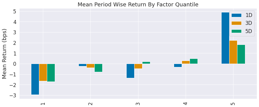
Returns Analysis

	1D	3D	5D
Ann. alpha	0.279	0.122	0.090
beta	0.104	0.043	0.050
Mean Period Wise Return Top Quantile (bps)	4.890	2.209	1.824
Mean Period Wise Return Bottom Quantile (bps)	-2.953	-1.651	-1.705
Mean Period Wise Spread (bps)	7.843	3.855	3.523

Information Analysis

	1D	3D	5D
IC Mean	0.016	0.012	0.016
IC Std.	0.173	0.169	0.169
Risk-Adjusted IC	0.091	0.068	0.098
t-stat(IC)	2.012	1.517	2.171
p-value(IC)	0.045	0.130	0.030
IC Skew	0.081	0.155	0.069
IC Kurtosis	0.342	0.335	0.409

Turnover Analysis

	1D	3D	5D
Quantile 1 Mean Turnover	0.347	0.601	0.788
Quantile 2 Mean Turnover	0.605	0.744	0.800
Quantile 3 Mean Turnover	0.652	0.763	0.786
Quantile 4 Mean Turnover	0.605	0.744	0.796
Quantile 5 Mean Turnover	0.350	0.596	0.781

	1D	3D	5D
Mean Factor Rank Autocorrelation	0.749	0.359	-0.016

<Figure size 432x288 with 0 Axes>

../_images/notebooks_pyfolio_integration_22_10.png

Run Pyfolio Analysis¶

Get Input Data¶

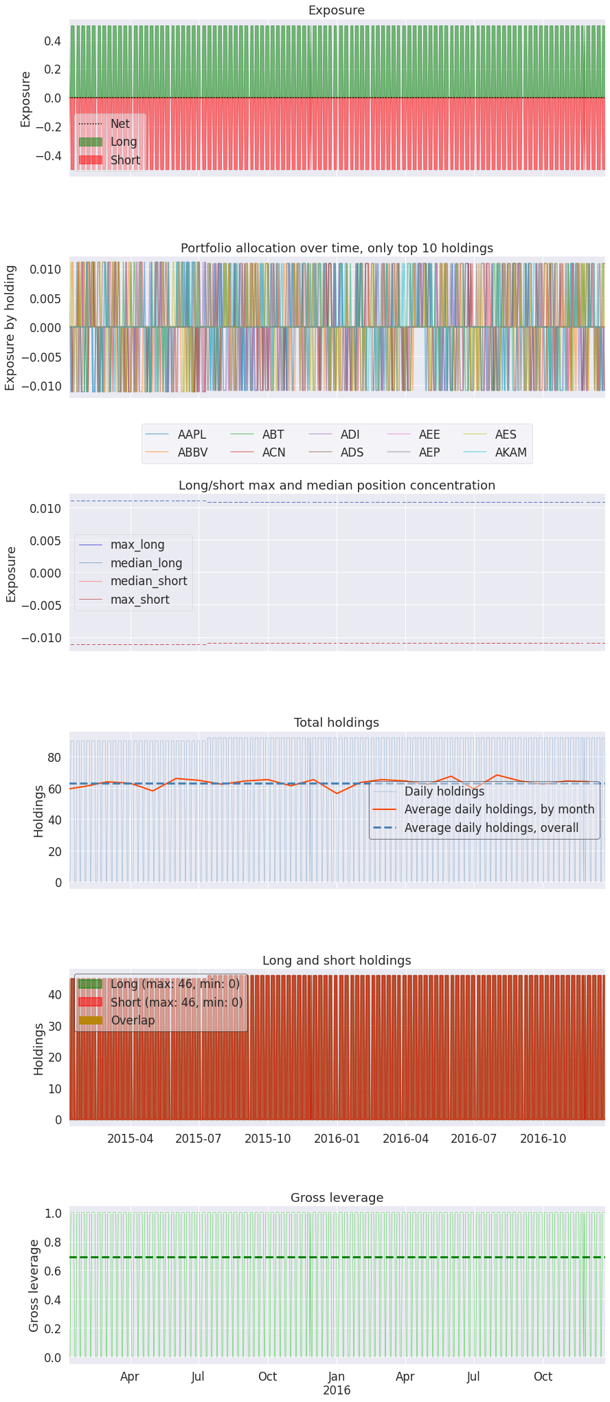
We can see in Alphalens analysis that quantiles 1 and 5 are the most predictive so we’ll build a portfolio data using only those quantiles.

[11]:

pf_returns, pf_positions, pf_benchmark = \
    alphalens.performance.create_pyfolio_input(factor_data,
                                               period='1D',
                                               capital=100000,
                                               long_short=True,
                                               group_neutral=False,
                                               equal_weight=True,
                                               quantiles=[1,5],
                                               groups=None,
                                               benchmark_period='1D')

Pyfolio Tearsheet¶

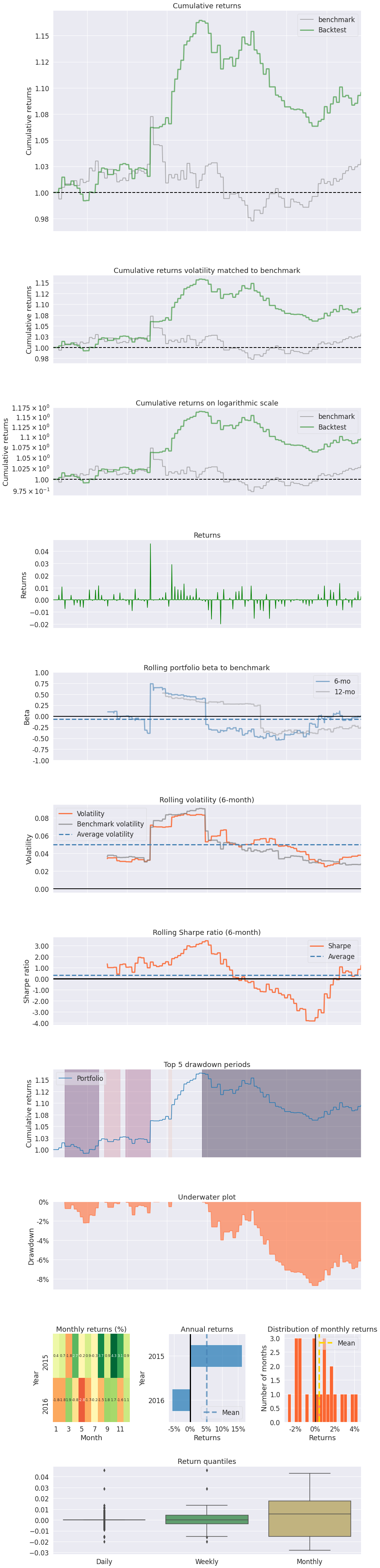
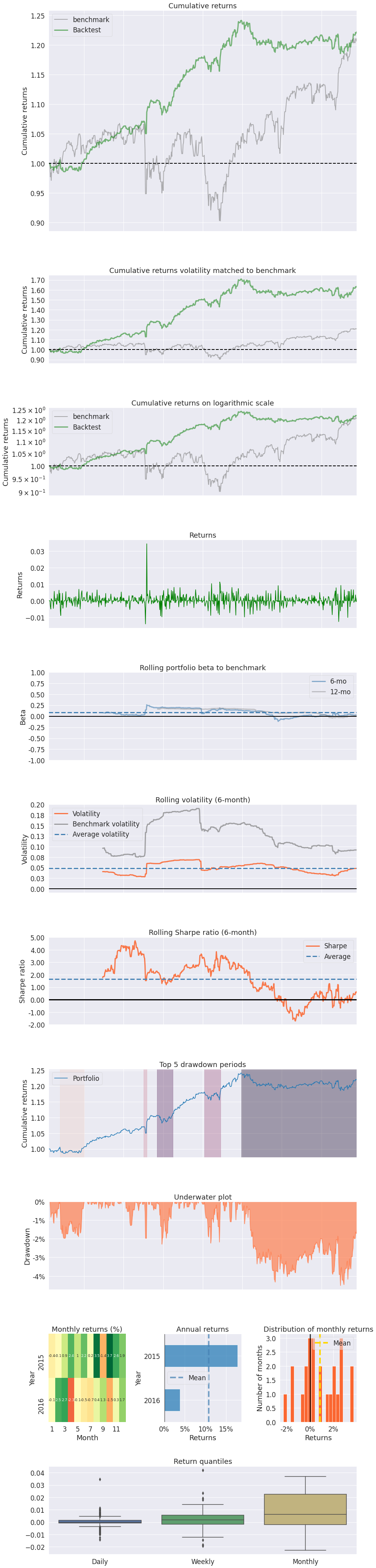
Now that we have prepared the data we can run Pyfolio functions

[12]:

pyfolio.tears.create_full_tear_sheet(pf_returns,
                                     positions=pf_positions,
                                     benchmark_rets=pf_benchmark)

	Backtest
Start date	2015-01-09
End date	2016-12-22
Total months	34
Annual return	7.349%
Cumulative returns	22.253%
Annual volatility	4.984%
Sharpe ratio	1.45
Calmar ratio	1.63
Stability	0.85
Max drawdown	-4.508%
Omega ratio	1.37
Sortino ratio	2.33
Skew	1.56
Kurtosis	21.29
Tail ratio	1.20
Daily value at risk	-0.599%
Gross leverage	0.69
Alpha	0.07
Beta	0.11

Worst drawdown periods	Net drawdown in %	Peak date	Valley date	Recovery date	Duration
0	4.51	2016-03-30	2016-11-14	NaT	NaN
1	2.29	2015-09-17	2015-09-28	2015-10-23	27
2	2.24	2016-01-04	2016-01-19	2016-02-11	29
3	1.97	2015-08-17	2015-08-21	2015-08-24	6
4	1.97	2015-02-04	2015-02-13	2015-04-01	41

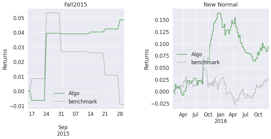
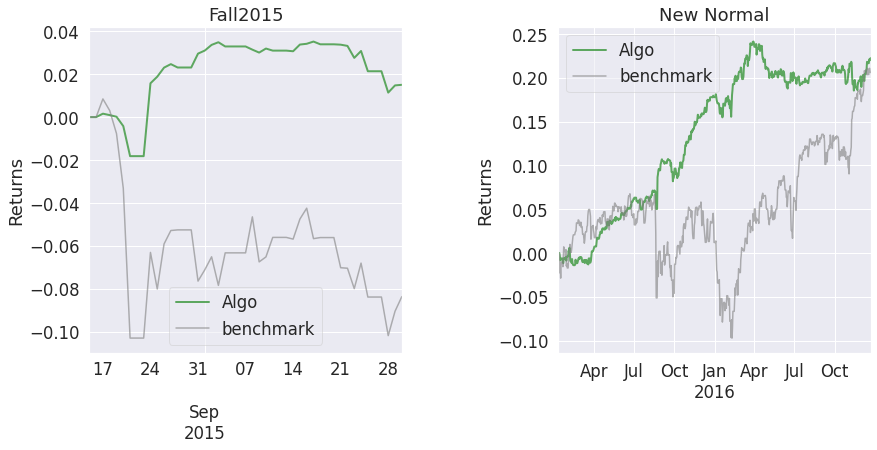
Stress Events	mean	min	max
Fall2015	0.03%	-1.40%	3.45%
New Normal	0.03%	-1.40%	3.45%

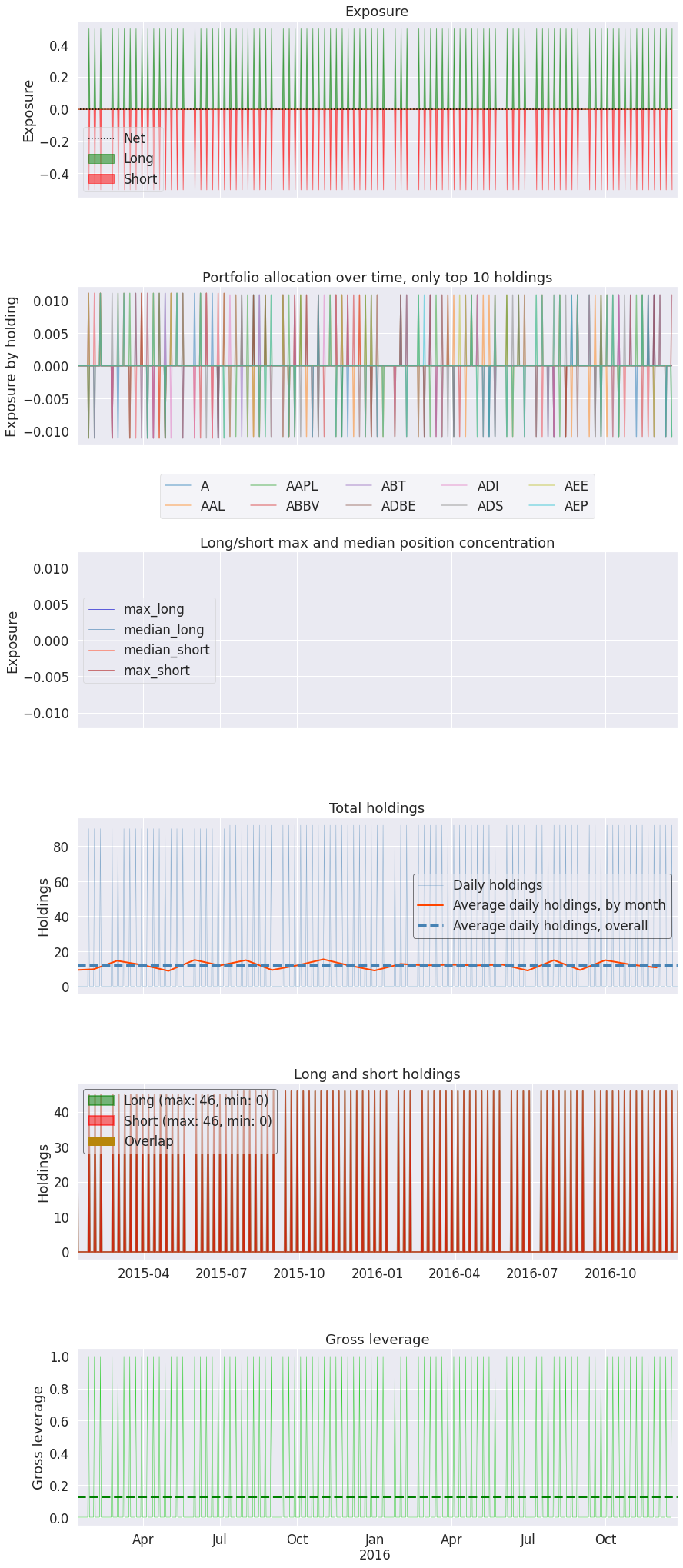
Top 10 long positions of all time	max
asset
ABBV	1.11%
ABT	1.11%
ACN	1.11%
ADS	1.11%
AEE	1.11%
AEP	1.11%
AES	1.11%
ALL	1.11%
AWK	1.11%
BSX	1.11%

Top 10 short positions of all time	max
asset
AAPL	-1.11%
ADI	-1.11%
AKAM	-1.11%
ALLE	-1.11%
AMD	-1.11%
ANSS	-1.11%
AON	-1.11%
ATVI	-1.11%
AVGO	-1.11%
AYI	-1.11%

Top 10 positions of all time	max
asset
AAPL	1.11%
ABBV	1.11%
ABT	1.11%
ACN	1.11%
ADI	1.11%
ADS	1.11%
AEE	1.11%
AEP	1.11%
AES	1.11%
AKAM	1.11%

../_images/notebooks_pyfolio_integration_29_6.png

../_images/notebooks_pyfolio_integration_29_7.png

../_images/notebooks_pyfolio_integration_29_8.png

Subset Performance¶

Weekday Analysis¶

Sometimes it might be useful to analyze subets of your factor data, for example it could be interesting to see the comparison of your factor in different days of the week. Below we’ll see how to select and analyze factor data corresponding to Mondays, the positions will be held the for a period of 5 days

[13]:

monday_factor_data = factor_data[ factor_data.index.get_level_values('date').weekday == 0 ]

[14]:

pf_returns, pf_positions, pf_benchmark = \
    alphalens.performance.create_pyfolio_input(monday_factor_data,
                                               period='5D',
                                               capital=100000,
                                               long_short=True,
                                               group_neutral=False,
                                               equal_weight=True,
                                               quantiles=[1,5],
                                               groups=None,
                                               benchmark_period='1D')

Pyfolio Tearsheet¶

[15]:

pyfolio.tears.create_full_tear_sheet(pf_returns,
                                     positions=pf_positions,
                                     benchmark_rets=pf_benchmark)

	Backtest
Start date	2015-01-12
End date	2016-12-19
Total months	33
Annual return	3.309%
Cumulative returns	9.578%
Annual volatility	5.058%
Sharpe ratio	0.67
Calmar ratio	0.38
Stability	0.37
Max drawdown	-8.687%
Omega ratio	1.40
Sortino ratio	1.23
Skew	4.96
Kurtosis	75.85
Tail ratio	1.73
Daily value at risk	-0.624%
Gross leverage	0.13
Alpha	0.03
Beta	0.17

Worst drawdown periods	Net drawdown in %	Peak date	Valley date	Recovery date	Duration
0	8.69	2015-12-20	2016-08-29	NaT	NaN
1	2.22	2015-02-08	2015-03-23	2015-04-27	56
2	1.40	2015-06-28	2015-07-13	2015-08-24	41
3	0.61	2015-05-10	2015-05-18	2015-06-15	26
4	0.54	2015-10-04	2015-10-05	2015-10-12	6

Stress Events	mean	min	max
Fall2015	0.10%	-0.64%	4.61%
New Normal	0.01%	-1.99%	4.61%

Top 10 long positions of all time	max
asset
A	1.11%
AAL	1.11%
ADBE	1.11%
ADI	1.11%
AEE	1.11%
AEP	1.11%
AET	1.11%
AIG	1.11%
AIZ	1.11%
ALLE	1.11%

Top 10 short positions of all time	max
asset
A	-1.11%
AAL	-1.11%
AAPL	-1.11%
ABBV	-1.11%
ABT	-1.11%
ADBE	-1.11%
ADI	-1.11%
ADS	-1.11%
AEE	-1.11%
AEP	-1.11%

Top 10 positions of all time	max
asset
A	1.11%
AAL	1.11%
AAPL	1.11%
ABBV	1.11%
ABT	1.11%
ADBE	1.11%
ADI	1.11%
ADS	1.11%
AEE	1.11%
AEP	1.11%

../_images/notebooks_pyfolio_integration_36_6.png

../_images/notebooks_pyfolio_integration_36_7.png

../_images/notebooks_pyfolio_integration_36_8.png

Pyfolio Integration¶

Imports & Settings¶

Load Data¶

YFinance Download¶

Data Formatting¶

Compute Factor¶

Run Alphalens Analysis¶

Get Input Data¶

Summary Tear Sheet¶

Run Pyfolio Analysis¶

Get Input Data¶

Pyfolio Tearsheet¶

Subset Performance¶

Weekday Analysis¶

Pyfolio Tearsheet¶